Many structured and unstructured systems - like organizations, molecules, social networks, or documents – can be represented quite naturally as graphs. In this article, we will explore ways on how we can make predictions and how to reason on such systems, specially on reasoning and understanding the documents.
First, let us see how a graph is defined. A graph represents the relations (graph edges) between a collection of entities (graph nodes). To fully describe a graph, we need to store the attributes of each node, each edge, and attributes of the entire graph.
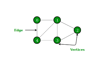
Figure 1 - Graph Example
V – collection of nodes’ attributes.
Example of node attribute: number of neighbors.
E – collection of edges attributes.
Example of edge attribute: edge weight.
U – global graph attributes.
Example: longest path, number of nodes.
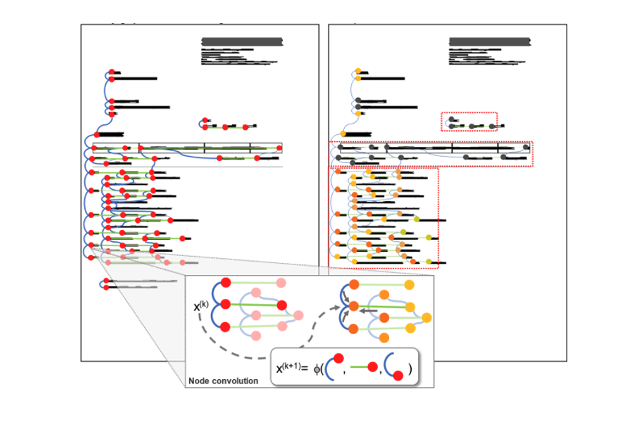
For example, we can define a document graph having text entities as nodes and relations between entities as edges. See below an example of how a document graph looks like. The set of nodes V corresponds to the detected entities of the document. The set of edges E represents visibility relations between nodes.
How can we reason and make predictions on a graph data?
First approach is to look at mechanisms that already have worked well in Machine Learning: neural networks have shown immense predictive power in a variety of learning tasks. However, neural networks have been traditionally used to operate on fixed-size and regular-structured inputs (such as text, images, and video). This makes them unable as they are to process graph-structured data.
The simplest GNN (Graph Neural Network) can be found in the framework proposed by Gilmer at al [1] using the Graph Nets architecture schematics introduced by Battaglia et al [2]. This type of GNN adopts a “graph-in, graph-out” architecture and is an optimizable transformation on all attributes of the graph (nodes, edges, global-context) that preserves graph symmetries (permutation invariances).
As can be seen in the diagram below, GNN uses a separate MLP (or any other differentiable model) on each component of a graph – U, V, E; we call this a GNN layer.
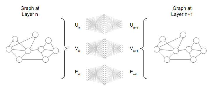
Stacking up all the GNN layers, we will obtain as output the transformed graph which contains embeddings for all the information from nodes, edges, and global context. It is important to notice that GNN does not alter the connectivity of the input graph, hence the output graph of a GNN will have the same adjacency list and the same number of features vector.
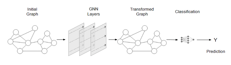
In the below diagram (Figure 4) can be seen how an end-to-end prediction with GNNs can looks like. In the case of invoice documents, these types of networks can predict if a node represents invoice date, invoice total amount or invoice currency.
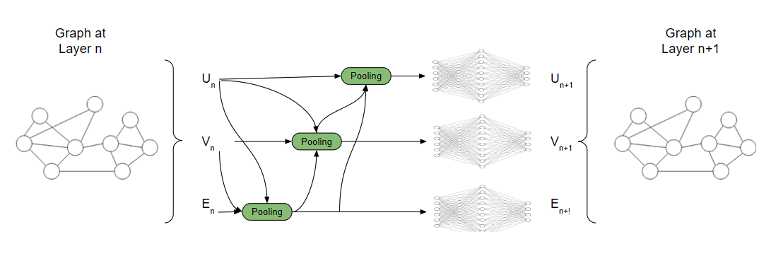
The example above is the simplest one, just to explain the concepts of GNN. We can observe that in this simple model, if we are doing predictions on the nodes from the graph, the model does not consider the information from edges and global context. Let’s improve this model to address this limitation and have GNN predictions by pooling information.
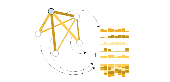
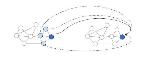
For instance, we want to collect information from edges and provide it to nodes for prediction. We can do this by pooling. Pooling proceeds in two steps:
- Step 1: for each item to be pooled, gather each of their embeddings and concatenate them into a matrix.
- Step 2: The gathered embeddings are then aggregated, usually via a sum operation.
By having this simple pooling approach established, the GNN layer represented in Figure 4 will be enhanced to more complex layer with three pooling functions. The new enhanced GNN layer is represented in figure 6.
There are various orders in which someone can update the information for nodes, edges and global context and the decision about choosing the right order is a design decision made when the product is built.
Now, let's try to improve even more the performance of our document reasoning model based on GNN. Convolutional Neural Networks (CNN) proved to be very powerful in extracting features from images. At the same time, we can look at the images as a graph with a very regular grid-like structure, where node attributes are RGB channel values. We can see in Figure 7 an example of how convolution in CNN works.
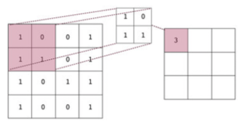
A natural idea will be to generalize convolutions to arbitrary graphs. The challenge we are facing here is ordinary convolutions are not node-order invariant, because they depend on the absolute positions of pixels.
We begin by introducing the idea of constructing polynomial filters over node neighborhoods, much like how CNNs compute localized filters over neighboring pixels. Let’s consider a graph G which has n nodes and A is the adjacency matrix of G. By definition, the graph Laplacian L is the square n x n matrix defined as L =D – A, where D is the diagonal degree matrix:

Now that we know what a graph Laplacian is, we can build polynomials of the form:
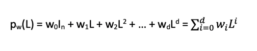
These polynomials can be seen as filters from the CNN. Each polynomial can be represented by its vector of coefficients w = [w0, w1, …, wd]. You can notice that pw(L) will be also a n x n matrix. To be able to improve even more the graph convolution, ChebNet (read more details in [4]) refines this idea of polynomial filters by looking at polynomial filters of the form:
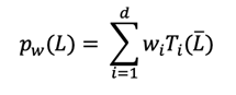
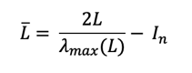
where Ti is the degree-i Chebyshev polynomial of the first kind and L is the normalized Laplacian defined using the largest eigenvalue of L:
The Chebyshev polynomials have certain interesting properties that make interpolation more numerically stable. We will not get into details here, but an interested read will find more in [4].
Based on the above filtering, the embedding computation algorithm becomes:

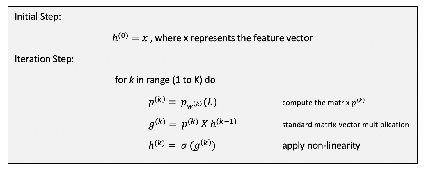
It is important to observe that this GNN layers reuse the same filter weight across all nodes, similar with weight sharing in CNN. In the algorithm above the h(k) node embeddings are computer while the w(k) weights are learnable parameters.
As shown before, the prediction will be a different neural network that will use as inputs the values of h(k) - where K represent the number of GNN layers. Therefore, the prediction for node v will be:
![]()
 Let us summarize what we learned so far:
- How to create a simple GNN network using basic GNN layers
- How to add pooling functions to improve the GNN, by collecting edge information and use it for node prediction
- How to replace the basic GNN layer with a more powerful convolution one (ChebNet)
At this moment, we have a pretty decent GNN model for reasoning on documents, having good results on node prediction. However, there are couple of models in the literature which are trying to improve the model even more. It is worth mentioning a few:
- Graph Convolutional Networks (GCN) (see [5])
- Graph Attention Networks
- Graph Sample and Aggregate (GraphSAGE)
- Graph Isomorphism Network
What we have presented in this article is just a starting point if someone wants to start and play with Machine Learning models for document reasoning and understanding. Of course, in production and real life such models are much more complex, also considering the language model and semantics, image of the analyzed document and images with parts of the documents, multi-head attention and many others.
If you want to develop your own document reasoning model for personal or academic purposes, please do not hesitate to contact Smart Touch Technologies for help and guidance.
Reference
[1] “Neural Message Passing for Quantum Chemistry” - J. Gilmer, S.S. Schoenholz, P.F. Riley, O. Vinyals, G.E. Dahl. Proceedings of the 34th International Conference on Machine Learning, Vol 70, pp. 1263--1272. PMLR. 2017.
[2] “Relational inductive biases, deep learning, and graph networks” - P.W. Battaglia, J.B. Hamrick, V. Bapst, A. Sanchez-Gonzalez, V. Zambaldi, M. Malinowski, A. Tacchetti, D. Raposo, A. Santoro, R. Faulkner, C. Gulcehre, F. Song, A. Ballard, J. Gilmer, G. Dahl, A. Vaswani, K. Allen, C. Nash, V. Langston, C. Dyer, N. Heess, D. Wierstra, P. Kohli, M. Botvinick, O. Vinyals, Y. Li, R. Pascanu. 2018.
[3] “Learning Convolutional Neural Networks for Graphs” - M. Niepert, M. Ahmed, K. Kutzkov. Proceedings of the 33rd International Conference on International Conference on Machine Learning - Volume 48, pp. 2014–2023. JMLR.org. 2016.
[4] “Convolutional Neural Networks on Graphs with Fast Localized Spectral Filtering” - M. Defferrard, X. Bresson, P. Vandergheynst. Advances in Neural Information Processing Systems, Vol 29, pp. 3844-3852. Curran Associates, Inc. 2016.
[5] “Semi-Supervised Classification with Graph Convolutional Networks” - T.N. Kipf, M. Welling. 5th International Conference on Learning Representations (ICLR) 2017, Toulon, France, April 24-26, 2017, Conference Track Proceedings. OpenReview.net. 2017.